Introduction to Python

Note: This lab note is still WIP, let me know if you encounter bugs or issues.

1. Introduction to Python

• 1.1 Powerful Statistical language: Python
• 1.2 Introduce Our Python Integrated Development Environment (IDE): Colab and Jupyter Notebooks

2. Preparations

• 2.1 Download and Installation
• 2.2 Jupter Notbook

3. Fundamentals

• 3.1 Before Coding
• 3.2 Use Python as Calculator
• 3.3 Data Structure: List and Data frame
• 3.4 Basic Plotting
• 3.5 Probability Distributions

Colab Notebook Open in Colab

1. Introduction to Python

1.1 Powerful Statistical language: Python

Python is a high-level, dynamically typed multiparadigm programming language. Python code is often said to be almost like pseudocode, since it allows you to express very powerful ideas in very few lines of code while being very readable.

• Python is universal.
• Python can do everything that R can do and much more.
• Python is very easy to learn and program in.

Where is it used?

Due to Python's ubiquity and portability, it is used in various applications like

• scientific computing,
• data science,
• artificial intelligence,
• text/data mining,
• web and software developments,
• task automation and many others.

Please visit this page for more applications of Python.

1.2 Colab and Jupyter Notebooks

Colab notebook

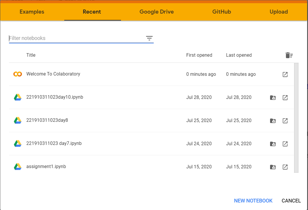
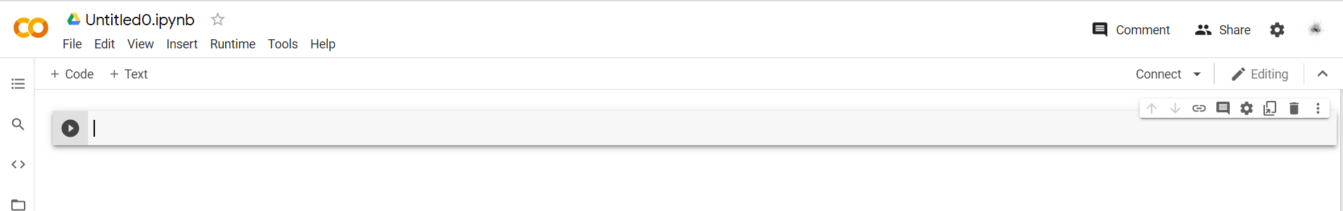
In 2018, Google launched an amazing platform called ‘Google Colaboratory’ (commonly known as ‘Google Colab’ or just ‘Colab’). Colab is an online cloud based platform based on the Jupyter Notebook framework, designed mainly for use in ML and deep learning operations.

Tensorflow + Keras + Colaboratory = Deep Learning Made Easy

Colab offers a free CPU/GPU quota and a preconfigured virtual machine instance set up for to run Tensorflow and Keras libraries using a Jupyter notebook instance.

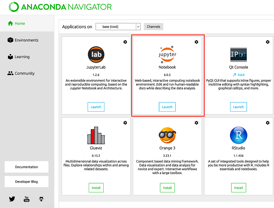
Jupyter notebook lets you write and execute Python code locally in your web browser. Jupyter notebooks make it very easy to tinker with code and execute it in bits and pieces; for this reason they are widely used in scientific computing.

2. Preparations

• 2.1 How to use Google Colab
• 2.2 Jupter Notbook (optional)

2.1 How to use Google Colab

Note: Useful intro about Colab

To start using Google Colab, you first have to log in to your Google account. Then click here to go to Google Colab’s home page.

The home screen of Google Colab will look like:

To open a new Python notebook, click ‘new notebook’ on the bottom right corner.

The opened notebook will look like:

A notebook named untitled0.iypnb is then created and automatically saved to your google drive.

Once it’s created, change the runtime by selecting changing runtime from runtime dropbox. Select Python 3 from the runtime type dropdown menu.

Now your notebook is ready to use!

• Checking Python Version

import sys              #only needed to determine Python version number
print('Python version ' + sys.version)

Python version 3.10.12 (main, Jun 11 2023, 05:26:28) [GCC 11.4.0]

You can check your Python version at the command line by running python --version

!python --version

Python 3.10.12

• Run Python in Colab Notebook

Enter the Hello World program and run it. Python is case-sensitive.

print("Hello, world!")

Hello, world!

• Importing a library that is not in Colaboratory

Most packages are included in the Colab that you installed. However, you will have to install other packages not included in Colab. To do this you will the !pip install <package-name> syntax in your Colab notebook:

# Install twitter package
!pip install tweepy
!pip install nltk

import tweepy
tweepy nltk

pip is the keyword that is used to install missing libraries/packages in Python.
Note: Useful intro about pip

2.2 Jupter Notbook (optional)

Which version of Python to use? Anaconda Version of Python has all the packages that we need. Anaconda distribution is a collection of Spyder, Jupyter Notebook, RStudio, and other commonly used scientific computing and data science tools. It is recommended for all the beginners to install Anaconda.

Step 1.Download and install Anaconda Python 3.7+ for your operating system here: https://www.anaconda.com/products/individual

Click Next >I agree> (Just Me) Next>(Choose destination folder ) next>(Register Anaconda as my default Python 3.X.XX) Install>Finish

After installation, launch the Anaconda Navigator, Jupyter Notebook, then create a Python 3 Notebook instance.

Then, click the Launch button below the Jupyter Notebook icon on the Navigator Home tab:

More info: https://docs.anaconda.com/anaconda/user-guide/getting-started/

Step 2. Figure out how to open a python shell in your environment. Test the Hello World program there. In Windows, it's probably as easy as running 'python' from the Windows menu. You'll have to verify that and troubleshoot it.

Checking Python Version

You can double-check your Python version at the command line after activating your environment by running python --version. For example, to check which version you are using, drop into Anaconda's terminal and type python --version.

• on my Windows box, I open Anaconda Prompt and type in:

  (base) C:\Users\XXXXX>python --version
  Python 3.7.13 :: Anaconda, Inc.

• On my Mac, I open iTerm and type in:

  ~XXXXX$ python --version
  Python 3.7.13 :: Anaconda, Inc.

Accessing help

Help in python on any topic involves

#Python help - This can be done on a (I)Python console
help(len)
?len

Help on built-in function len in module builtins:

len(obj, /)
    Return the number of items in a container.

3. Fundamentals

3.1 Before Coding

• To start using Google Colab, you first have to log in to your Google account.
• To open a new Python notebook, click ‘new notebook’ on the bottom right corner.
• Rename a nnotebook named untitled0.iypnb
• Now your notebook is ready to use.

3.2 Use Python as Calculator

x=10
y = 5
x+y

15

# Python program explaining
# log() function
import numpy as np
out = np.log(10)
print (round(out,6))

2.302585

# importing "math" for mathematical operations
import math

# Printing the log base 10 of 10
print ("Logarithm base 10 of 10 is : ", end="")
print (math.log10(10))

Logarithm base 10 of 10 is : 1.0

exponent =5
out = math.exp(exponent)
print (round(out,4))

148.4132

# Python code to demonstrate the working of cos()
x=10
out=math.cos(x)
print (round(out,6))

-0.839072

Booleans: Python implements all of the usual operators for Boolean logic, but uses English words rather than symbols (==, >, <,&&, ||, etc.):

x==y

False

x>y

True

3.3 Data Structure: List and Data frame

3.3.1 List

A list is the Python equivalent of an array, but is resizeable and can contain elements of different types.

A common data type in R is the vector. Python has a similar data type, the list. In Python, vector is a single one-dimension array of lists and behaves same as a Python list.

R vs Python: Different similarities and similar difference

# Python lists
a=[4,5,1,3,4,5]
print(a[2])
print(a[2:5])
print(type(a))
# Length of a
print(len(a))

1
[1, 3, 4]
<class 'list'>
6

xs = [3, 1, 2]   # Create a list
print(xs, xs[2])  # Prints "[3, 1, 2] 2"
print(xs[-1])     # Negative indices count from the end of the list; prints "2"

[3, 1, 2] 2
2

xs[2] = 'foo'    # Lists can contain elements of different types
print(xs)         # Prints "[3, 1, 'foo']"

[3, 1, 'foo']

xs.append('bar') # Add a new element to the end of the list
print(xs)   # Prints "[3, 1, 'foo', 'bar']"

[3, 1, 'foo', 'bar']

x = xs.pop()     # Remove and return the last element of the list
print(x, xs)      # Prints "bar [3, 1, 'foo']"

bar [3, 1, 'foo']

mylist=[x, xs, cars]
mylist

More info: https://docs.python.org/3.5/tutorial/datastructures.html#more-on-lists

Slicing: In addition to accessing list elements one at a time, Python provides concise syntax to access sublists; this is known as slicing:

nums = list(range(5))     # range is a built-in function that creates a list of integers
print(nums)               # Prints "[0, 1, 2, 3, 4]"
print(nums[2:4])          # Get a slice from index 2 to 4 (exclusive); prints "[2, 3]"
print(nums[2:])           # Get a slice from index 2 to the end; prints "[2, 3, 4]"
print(nums[:2])           # Get a slice from the start to index 2 (exclusive); prints "[0, 1]"
print(nums[:])            # Get a slice of the whole list; prints "[0, 1, 2, 3, 4]"
print(nums[:-1])          # Slice indices can be negative; prints "[0, 1, 2, 3]"
nums[2:4] = [8, 9]        # Assign a new sublist to a slice
print(nums)

[0, 1, 2, 3, 4]
[2, 3]
[2, 3, 4]
[0, 1]
[0, 1, 2, 3, 4]
[0, 1, 2, 3]
[0, 1, 8, 9, 4]

import numpy as np
a =[5,2,3,1,7]
b =[1,5,4,6,8]
a=np.array(a)
b=np.array(b)
#Element wise addition
print(a+b)
#Element wise subtraction
print(a-b)
#Element wise product
print(a*b)
# Exponentiating the elements of a list
print(a**2)

[ 6  7  7  7 15]
[ 4 -3 -1 -5 -1]
[ 5 10 12  6 56]
[25  4  9  1 49]

3.3.2 Data frames

For Python we need to use the Pandas package. Pandas is quite comprehensive in the list of things we can do with data frames The most common operations on a dataframe are

• Check the size of the dataframe
• Take a look at the top 5 or bottom 5 rows of dataframe
• Check the content of the dataframe

#Python
import sklearn as sklearn
import pandas as pd
from sklearn import datasets
# This creates a Sklearn bunch
data = datasets.load_iris()
# Convert to Pandas dataframe
iris = pd.DataFrame(data.data, columns=data.feature_names)
iris

	sepal length (cm)	sepal width (cm)	petal length (cm)	petal width (cm)
0	5.1	3.5	1.4	0.2
1	4.9	3.0	1.4	0.2
2	4.7	3.2	1.3	0.2
3	4.6	3.1	1.5	0.2
4	5.0	3.6	1.4	0.2
...	...	...	...	...
145	6.7	3.0	5.2	2.3
146	6.3	2.5	5.0	1.9
147	6.5	3.0	5.2	2.0
148	6.2	3.4	5.4	2.3
149	5.9	3.0	5.1	1.8

150 rows × 4 columns

a. Size

For Python use .shape

#Python - size
import sklearn as sklearn
import pandas as pd
from sklearn import datasets
data = datasets.load_iris()
# Convert to Pandas dataframe
iris = pd.DataFrame(data.data, columns=data.feature_names)
iris.shape

(150, 4)

b. Top & bottom 5 rows of dataframe

To know the top and bottom rows of a data frame we use head() & tail as shown below for Python

#Python
data = datasets.load_iris()
# Convert to Pandas dataframe
iris = pd.DataFrame(data.data, columns=data.feature_names)
print(iris.head(5))
print(iris.tail(5))

   sepal length (cm)  sepal width (cm)  petal length (cm)  petal width (cm)
0                5.1               3.5                1.4               0.2
1                4.9               3.0                1.4               0.2
2                4.7               3.2                1.3               0.2
3                4.6               3.1                1.5               0.2
4                5.0               3.6                1.4               0.2
     sepal length (cm)  sepal width (cm)  petal length (cm)  petal width (cm)
145                6.7               3.0                5.2               2.3
146                6.3               2.5                5.0               1.9
147                6.5               3.0                5.2               2.0
148                6.2               3.4                5.4               2.3
149                5.9               3.0                5.1               1.8

c. Check the content of the dataframe

#Python
data = datasets.load_iris()
# Convert to Pandas dataframe
iris = pd.DataFrame(data.data, columns=data.feature_names)
print(iris.info())

<class 'pandas.core.frame.DataFrame'>
RangeIndex: 150 entries, 0 to 149
Data columns (total 4 columns):
 #   Column             Non-Null Count  Dtype  
---  ------             --------------  -----  
 0   sepal length (cm)  150 non-null    float64
 1   sepal width (cm)   150 non-null    float64
 2   petal length (cm)  150 non-null    float64
 3   petal width (cm)   150 non-null    float64
dtypes: float64(4)
memory usage: 4.8 KB
None

d. Check column names

#Python
data = datasets.load_iris()
# Convert to Pandas dataframe
iris = pd.DataFrame(data.data, columns=data.feature_names)
#Get column names
print(iris.columns)
## Index(['sepal length

Index(['sepal length (cm)', 'sepal width (cm)', 'petal length (cm)',
       'petal width (cm)'],
      dtype='object')

e. Rename columns

In Python we can assign a list to s.columns

#Python
data = datasets.load_iris()
# Convert to Pandas dataframe
iris = pd.DataFrame(data.data, columns=data.feature_names)
iris.columns = ["lengthOfSepal","widthOfSepal","lengthOfPetal","widthOfPetal"]
print(iris.columns)

Index(['lengthOfSepal', 'widthOfSepal', 'lengthOfPetal', 'widthOfPetal'], dtype='object')

f.Details of dataframe

#Python
data = datasets.load_iris()
# Convert to Pandas dataframe
iris = pd.DataFrame(data.data, columns=data.feature_names)
print(iris.info())

<class 'pandas.core.frame.DataFrame'>
RangeIndex: 150 entries, 0 to 149
Data columns (total 4 columns):
 #   Column             Non-Null Count  Dtype  
---  ------             --------------  -----  
 0   sepal length (cm)  150 non-null    float64
 1   sepal width (cm)   150 non-null    float64
 2   petal length (cm)  150 non-null    float64
 3   petal width (cm)   150 non-null    float64
dtypes: float64(4)
memory usage: 4.8 KB
None

g. Subsetting dataframes

#Python
# To select an entire row we use .iloc. The index can be used with the ':'. If
# .iloc[start row: end row]. If start row is omitted then it implies the beginning of
# data frame, if end row is omitted then it implies all rows till end
#Python
data = datasets.load_iris()
# Convert to Pandas dataframe
iris = pd.DataFrame(data.data, columns=data.feature_names)
print(iris.iloc[3])
print(iris[:5])
# In python we can select columns by column name as follows
print(iris['sepal length (cm)'][2:6])
#If you want to select more than 2 columns then you must use the double '[[]]' since the
# index is a list itself
print(iris[['sepal length (cm)','sepal width (cm)']][4:7])

sepal length (cm)    4.6
sepal width (cm)     3.1
petal length (cm)    1.5
petal width (cm)     0.2
Name: 3, dtype: float64
   sepal length (cm)  sepal width (cm)  petal length (cm)  petal width (cm)
0                5.1               3.5                1.4               0.2
1                4.9               3.0                1.4               0.2
2                4.7               3.2                1.3               0.2
3                4.6               3.1                1.5               0.2
4                5.0               3.6                1.4               0.2
2    4.7
3    4.6
4    5.0
5    5.4
Name: sepal length (cm), dtype: float64
   sepal length (cm)  sepal width (cm)
4                5.0               3.6
5                5.4               3.9
6                4.6               3.4

h. Computing Mean, Standard deviation, Max, Min and Median

#Python
data = datasets.load_iris()
# Convert to Pandas dataframe
iris = pd.DataFrame(data.data, columns=data.feature_names)
print(round(iris['sepal length (cm)'].mean(),2)) #Mean
print(round(iris['sepal width (cm)'].std(),2))#Standard deviation
print(round(iris['sepal length (cm)'].max(),2))
print(round(iris['sepal length (cm)'].min(),2))
print(round(iris['sepal length (cm)'].median(),2))

5.84
0.44
7.9
4.3
5.8

3.4 Basic Plotting

• Upload CSV file manually

# Upload local file to Colab notebook
from google.colab import files
import pandas as pd
uploaded = files.upload()

Upload widget is only available when the cell has been executed in the current browser session. Please rerun this cell to enable.

Saving cars.csv to cars.csv

Note: It will prompt you to select a file. Click on “Choose Files” then select and upload the file. Wait for the file to be 100% uploaded. You should see the name of the file once Colab has uploaded it.

• Matplotlib is a plotting library.
  • Plotting
  • The most important function in matplotlib is plot, which allows you to plot 2D data.
  • Here is a simple example.

# Plot the points using matplotlib
# If you don't use Colab, you can read using read_csv() from Pandas
import matplotlib.pyplot as plt
import io
cars= pd.read_csv(io.BytesIO(uploaded['cars.csv']))
plt.scatter(cars['speed'],cars['dist'])
plt.title('Scatter plot')
plt.xlabel('speed')
plt.ylabel('distance')
plt.show()

3.5 Probability Distributions

Types of distributions: norm, binom, beta, cauchy, chisq, gamma, geom, hyper, lnorm, logis, nbinom, t, unif, weibull, wilcox, etc.

Four prefixes:

• ‘pdf’ for probability density function (PDF)

• ‘pmf’ for probability mass function (PMF)

• ‘cdf’ for distribution (CDF)

• ‘ppf’ for quantile (Percentiles)

• ‘rvs’ for random generation (Simulation)

# Python: random seed; use rondom function.
# If the replication needs, it's better to read in the data
import random
random.seed(1234)

Note: random number sequences in Python and R are not the same even using the same random seed. To create same random number sequence in Python and R, you can use a C-based program called SyncRNG: https://github.com/GjjvdBurg/SyncRNG

# call scipy.stats library
# import binom distribution
# round 5 decimals
from scipy.stats import binom,norm
x, n, p=4,10,0.5
round(binom.pmf(x, n, p),5)

0.20508

round(norm.cdf(1.86),5)

0.96856

round(norm.ppf(0.975),5)

1.95996

norm.rvs(size=10)

array([ 1.03133057,  0.9641532 , -1.14807617, -0.90139219,  1.53622188,
       -0.5087218 ,  2.32006624,  0.27640445, -0.67003179, -1.0523237 ])

# generate random numbers from N(100,20)
# The location (loc) keyword specifies the mean. The scale (scale) keyword specifies the standard deviation.
data_normal= norm.rvs(size=10,loc=100,scale=20)

%%shell
jupyter nbconvert --to html ///content/1A.Introduction_to_Python.ipynb